Schroeder Integration and Reverberation Time

Schroeder proposed a new method to calculate reverberation time using backward integration. The proposed method allows a more accurate estimation of the reverberation and has become a standard technique to compute the acoustic parameter.
Consider an impulse response h(n). The decay curve of the acoustic energy $p^2$ is defined as

$\left\langle p^2(t)\right\rangle=N\int_t^\infty h^2(\tau)\,\text{d}\tau$

where N power per unit bandwidth. This mathematical relation takes advantage of the ensemble average being equal to the backward integration of the squared impulse response. Translating to discrete-time, the backward integration becomes a cumulative sum of the energy. The ensemble average represents an infinite number of measurements, increasing the accuracy of the estimation.

After calculating the energy decay curve, linear regression may be applied to the curve to approximate the reverberation time of the acoustic space. Acoustic parameters T10, T20, T30 are often used due to the inability to have a full decay of -60 dB, which is one-millionth of the initial value. A more robust regression may also be utilized. A nonlinear linear model proposed by Xiang uses

$D(k) = x_0(t_K+t_k)+x_1 \text{e}^{-x_2t_k}$

where the first term models the noise and the second term models the signal-rate slope. Although the fit works well in noisy conditions, the model’s convergence relies heavily on a well estimated initial guess. Finally, variable $x_2$ is used to calculate reverberation time:

$RT=\frac{13.8}{x_2}$

Figure 1. Example backward integration. (Left) Impulse Response. (Right) Energy time function in blue with the
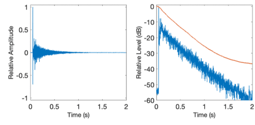
decay curve calculated using backward integration.

Complete Communications Engineering