Interpolation with an Ideal FIR Filter

Interpolation is the process of estimating unknown values of a signal given a set of known values of the same signal. Interpolation essentially is able to estimate particular missing data points by taking a weighted average of nearby given data points. Applications of interpolation include (but are not limited to) D/A conversion, sampling rate conversion, signal restoration, and fractional delay filters.

Mathematically, interpolation can be modeled by the block diagram system below.

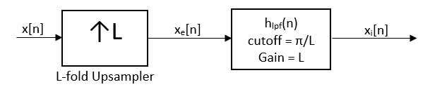
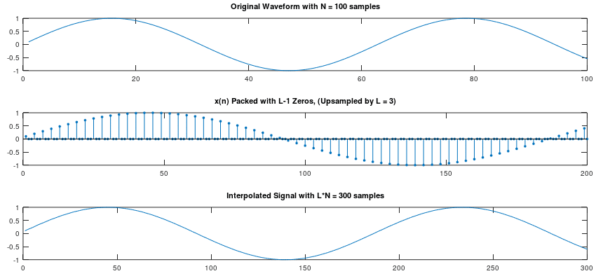
A given discrete signal x[n] must first be upsampled to zero-pack the signal with L-1 zeros. Zero-packing is simply the process of inserting zeros in between the samples of x[n]. The resulting signal $x_e(n)$ will have L times as many samples as the original signal x(n). Upsampling can be described mathematically as:

$x_e(n) = \sum_{k = \infty }^{\infty } x[k]\delta [n-kL]$ (1.1)

Subsequently, the upsampled signal xe[n] must be convolved with the impulse response of a low-pass filter with cutoff frequency $|\omega_{c} | = \pi /L$ , and gain L. The equation for the ideal low-pass filter with cutoff $|\omega_{c} | = \pi /L$ and gain L is given as:

$h_{lpf} = (n) = \frac{1}{2\pi }\int_{\omega _{c}}^{\omega _{c}}Le^{j\omega n}d\omega = \frac{sin(\pi n/L))}{\pi n/L}$ (1.2)

By performing the following convolution, the upsampled signal is interpolated to obtain$latex<\x_i[n]>$. Given a signal x[n] with N total samples, the interpolated signal xi[n] will have N*L total samples. Figure 1 on the following page demonstrates the application of interpolation on a sinusoidal waveform. Note that, in order to perfectly reconstruct the ideal desired signal, an infinite amount of filter taps must be used.

$x_{i}(n) = h_{lpf}[n]*x_{e}[n] = \sum_{k = -\infty }^{\infty }x_{e}[k]h_{i}[n-k] = \sum_{k = -\infty }^{\infty }x_{e}[k] sinc[\pi (n-k)/L]$ (1.3)

Figure 1: Interpolation of a Sinusoidal Waveform with L = 3

Complete Communications Engineering