The Transversal Wiener Filter

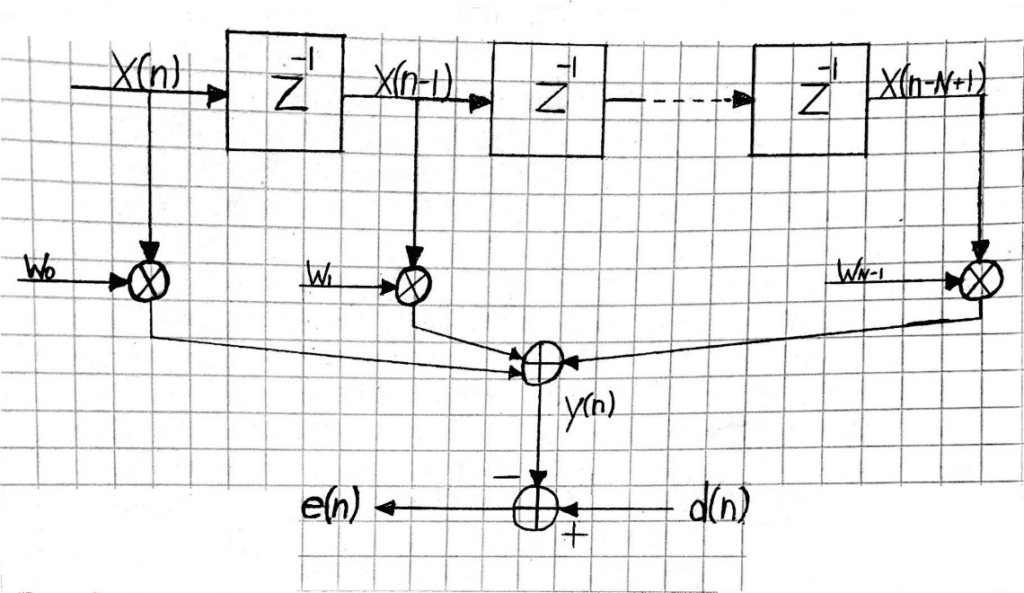
Wiener filter theory forms the basis upon which many different adaptive signal processing applications are designed. Common applications which implement Wiener filter theory include linear predication, noise filtering, and echo cancellation. In general, Wiener filters attempt to calculate a statistical estimate of a desired signal using the mean square error criterion. To demonstrate, consider a FIR transversal Wiener filter with filter tap vector $w = \left [ w_{0}, w_{1}, \cdots, w_{N-1} \right ]$ and input vector $\mathbf{x} = \left [ x(n), x(n-1), \cdots, x(n-N+1) \right ]$ .

Figure 1: Transversal Wiener Filter

The transversal Wiener filter output y(n) is given as:

$y(n) = \sum_{i = 0}^{N-1}w_{i}x(n-i) = \mathbf{w}^{T}\mathbf{x}(n)$ (1.1)

with error e(n) in terms of output y(n) and desired signal d(n):

$e(n) = d(n) - y(n) = d(n) - \mathbf{w}^{T}\mathbf{x}(n)$ (1.2)

The mean square error in the case of the transverse Wiener filter may be written as:

$\xi = E\left [ e^{2}(n) \right ] = E\left [ (d(n) - \mathbf{w}^{T}\mathbf{x}(n))^{2} \right ]$ (1.3)

$= E\left [ d^{2}(n) \right ] - \mathbf{w}^{T}E\left [ \mathbf{x}(n)d(n) \right ] - E[d(n)\mathbf{x}^{T}(n)]\mathbf{w} + \mathbf{w}^{T}E\left [\mathbf{x}(n)\mathbf{x}^{T}(n) \right ]\mathbf{w}$

Let the cross-correlation vector $\mathbf{p}$ and the autocorrelation vector $\mathbf{R}$ be defined as the following:

$\mathbf{p} = E\left [ \mathbf{x}(n)d(n) \right ]$
$\mathbf{R} = E\left [ \mathbf{x}(n)\mathbf{x}^{T}(n) \right ]$

Substituting in the previous equations to eq. 1.3, the mean square error can be written as:

$\xi = E[d^{2}(n)] - 2\mathbf{w}^{T}\mathbf{p} +\mathbf{w}^{T}\mathbf{R}\mathbf{w}$ (1.4)

To obtain the optimal solution, the performance functional must be minimized by equating the gradient of the mean square error to zero:

$\bigtriangledown \xi = \left [ \frac{\partial \xi }{\partial w_{0}} ,\frac{\partial \xi }{\partial w_{1}}, \cdots, \frac{\partial \xi }{\partial w_{N-1}} \right ] = 0$

$\bigtriangledown \xi = 0 = 2\mathbf{Rw}-2\mathbf{p}$

Therefore, eq. 1.4 is then translated into the solution to the Wiener-Hopf equation:

$\mathbf{w} = \mathbf{R}^{-1}\mathbf{p}$ (1.5)

The minimum mean square error criterion is satisfied when the optimal coefficients for the transversal Wiener filter are calculated from the Wiener-Hopf equation (eq. 1.5). Therefore, substituting eq. 1.5 into eq. 1.4, the minimum mean square error may be obtained as follows:

$\xi_{min} = E\left [ d^{2}(n) \right ] - \mathbf{p}^{T}\mathbf{R}^{-1}\mathbf{p}$ (1.6)

Using the mean square error performance function results in a solution which is both mathematically tractable and unambiguous. Simply put, it is mathematically practical to obtain a closed form solution. For FIR filters, a singular global minimum is guaranteed for the mean square error performance function. Thus, there is an objective optimum solution to the Wiener-Hopf equation. In general, IIR filters may result in performance functionals which have several minima. Because of this, FIR filters are much more prevalent in adaptive filtering applications than IIR filters.

Complete Communications Engineering