The Simple Theory of Noise Reduction: Wiener Filtering

The noise reduction problem can be described by the following simple diagram below.

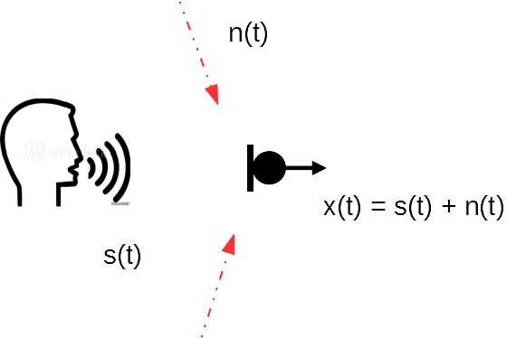
Figure 1: A Simple Case for Noise Reduction

Noises are everywhere. Figure 1 describes a scenario that a person is talking into a microphone. The microphone captures a sound,

$x\left(t\right)\ =\ s(t)\ +\ n(t)$

where s(t) is the person’s speech signal, n(t) is the total contribution of all noises around the microphone.

The problem of noise reduction can be simply stated as below:

Given the captured signal x(t), how to recover s(t) in some sense of optimality.

We reformate the problem into the following optimization problem:

$x\left(t\right)\ =\ s(t)\ +\ n(t)$

and we assume that the recovered speech is

$\hat{s}\left(t\right)=w\ast\ x\left(t\right)$

By some simple mathematics, we can derive the following,

$w=\frac{E\left[s\left(t\right)^2\right]}{E\left[x\left(t\right)^2\right]}$

This gives the famous Wiener filtering solution,

$\hat{s}\left(t\right)=w\ast\ x\left(t\right)$ = $\frac{E\left[s\left(t\right)^2\right]}{E\left[x\left(t\right)^2\right]}\ x(t)$ (Eq. 5)

A variety of different modifications has been added to this simple solution in practice. However, the root of almost all noise reduction algorithms can be traced to this beautiful but extremely simple solution in Equation (5).

Complete Communications Engineering