Data Modeling

In signal processing, we are often given a sequence of sample data and asked to analyze features or patterns of the data sequence. A basic tool is to represent the data sequence into some parametric model. The fundamental assumption is that the data sequence given is considered as a realization of a stationary random process. The moments of the random process are time invariant.

Basic Framework of Data Modeling

To simplify the explanation, we divide the data modeling processing into the following steps.

• Data sequence is assumed to fit the following hypothetical model as shown in Figure 1.
• All second moment statistics are known
• Derive the set of equations whose solution provides the model parameters as shown in Figure 1.

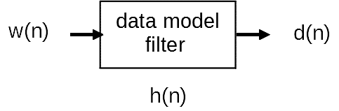
Figure 1 Parametric Data Modeling

We assume that the input $q(n)$ is white and the output $d(n)$ is statistically equivalent to the data sequence given. Our goal is to derive the parameters that describe the data model filter $h(n)$ based only on the given data.

Let us assume that $w(n)$ is white with power density $\sigma_{w}^{2}$ , the power spectrum density of $d(n)$ can be represented as

$Pd (f)=\left | H(f) \right | ^{2} Pw (f)=\sigma_w^{2} \left | H(f)\right |^{2}$

It seems that any desired second moment characteristics can be produced by applying white noise to an appropriate linear filter!

The design of the linear filter to represent a random process with some desired power density spectrum or correlation function is referred to as signal modeling. The procedure may also be used to reproduce the random process and the reproduction process is usually referred to as signal synthesis. It is apparent that the same techniques can be developed to perform both tasks.

We consider cases that $H(z)$ is rational polynomial only. The following three types are commonly used.

Type of Models

• Autoregressive (AR): it is an all pole filter with all zeroes at the origin. AR model is relatively easy to design. The equations that determine its parameters are linear.
• Moving average (MA): it is an all zero filter with all poles. Its design can be more involved than it looks.
• Autoregressive moving average (ARMA): it is a pole-zero filter. The model is the most flexible and often requires fewer parameters to match a desired power spectrum density function. However, ARMA design is often more difficult than either AR or MA.

Complete Communications Engineering

Data Modeling

Basic Framework of Data Modeling

Type of Models