Circular Microphone Array

Figure 1 shows a typical circular microphone array configuration. N microphones are positioned on the perimeter of a circle and one at the center. The radius of the circle is d.

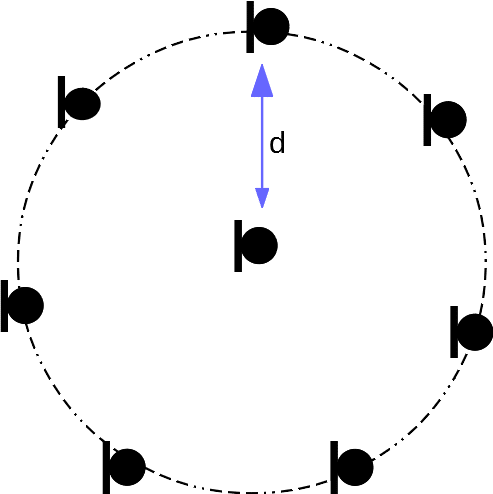
We name the center microphone as microphone number 0, and the others are arbitrarily labeled from 1 to M, clockwise.

1. Circular Microphone Array

The size of the array determines the sampling field of the array in the sound field. The radius of the array can range from a few center meters to meters. The reference design from Texas Instrument, TIDA-01454, has a radius 24 mm with a total of 8 microphones.

If the Texas Instrument circular array is used as a ceiling application, the following diagram shows the effective delay between the center microphone and one of the side microphones.

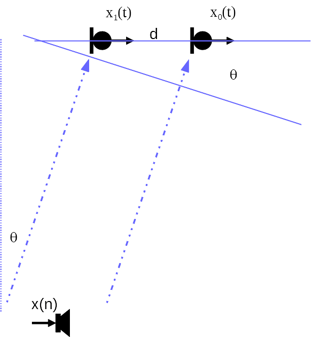
The effective distance in the sound propagation direction between microphone 1 and the center reference microphone would be much shorter than the actual radius of the array. The time delay of the sound wave front reaches to the two microphones will be

ΔT=dsinθ/c

For d = 24,  is at 30-degree angle, we will have roughly 0.03 millisecond delay, equivalent to about half a sample delay at sampling frequency 16kHz.

2. Why acoustic array is so difficult?

There are two main issues with using this microphone array, 1) the spatial resolution, 2) reflections.

Spatial resolution of an array is defined as the capability that the array can distinguish the different angles of two incoming sound waves. An array resolves the incoming angle of the sound wave through measuring and comparing the time of arrivals of the incoming signal. The farther apart of the microphones, the more accurate the delay measurement would be. In this specific circular microphone design, the maximum delay that can be measured in a planar model would be 0.06miliseconds, or roughly one sample for a sound signal sampled at 16kHz.

The second problem is the multiple reflections. The most favorable environment for using beamforming technology is free space, where sounds travel free from reflectors. Reflectors present multiple different incoming directions in spatial dimension in addition to the different time-of-arrivals in the time domain. The added complexity makes it difficult for an algorithm resolve incoming directions.

3. Wideband Microphone Array Optimum Implementation

In free space, a single sound source creates a single sound wave impinging on the microphone array in one spatial direction. As shown in Figure 2, the angle is shown as . However, when reflectors are around the microphone array, there will be multiple reflections for the same sound source. Therefore, a single delay with a direction will be an accurate model of the problem. Multiple pairs of delay and direction, ( i,  ), should be used instead.

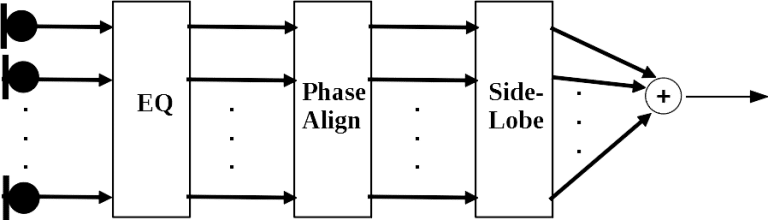
Based on the multiple reflection model, the following steps would be theoretically optimum.

1. line up each sound source in the time domain first, as represented by the first block (EQ), for each microphone for each incoming sound source. This procedure is equivalent to channel equalization in communication or dereverberation
2. After each sound source on each microphone is equalized or dereverberated, a coherent combining for each sound source on all the microphones can be phase-aligned
3. When all sources are time equalized and spatially phase aligned on each for the microphone, a weight set can be applied to every microphone to design a spatial window filter to control the spatial side lobe of the beamformer.
4. The above three steps complete all the necessary processing on each microphone and spatial filtering with the designed spatial filter weights can be applied to obtain the beamforming result, which is a one-dimensional time domain signal
5. Single channel filtering can be further applied to the beamforming result to further reduce noise or as a post processing step to reduce artifacts

The above steps if perfectly carried out would result in a close to optimum beamforming solution.

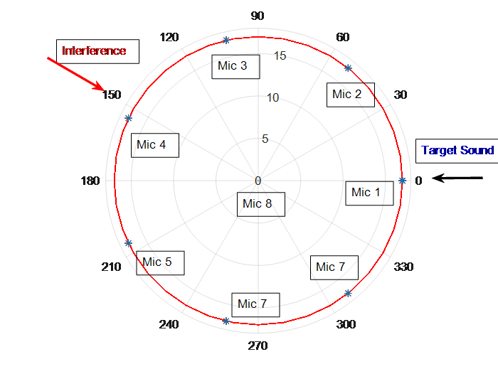
Figure 4 Circular Array Configuration and Sound Source Locations

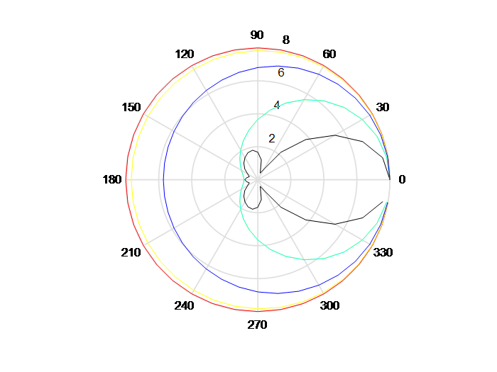
Figure 5 Beam Pattern for Desired Target at 0 Degree

Figure 4 shows a hypothetic target and interference configuration. Figure 5 shows the frequency dependence of the directional gain of the circular array. The beam patterns from inside out are for frequencies at 8k, 4k, 2k, 1k, and 200Hz. We assume the desired sound source is at exactly 0-degree angle. The array has good directional suppression at the opposite direction, 180 degree, for frequencies over 4kHz but very little suppression for below 2kHz.