Acoustic Echo Cancellation With The ML Algorithm

Typical algorithms for acoustic echo cancellation (AEC) are the LMS and NLMS algorithms for their ease of implementation and relatively fast convergence rates, especially for real time implementations. The filter taps obtained from the NLMS, and by extension the LMS algorithm, is however not the maximum likelihood estimate. We derive the maximum likelihood estimate and compare to the NLMS and the LMS algorithms. Consider the systems depicted in Figure 1 below:

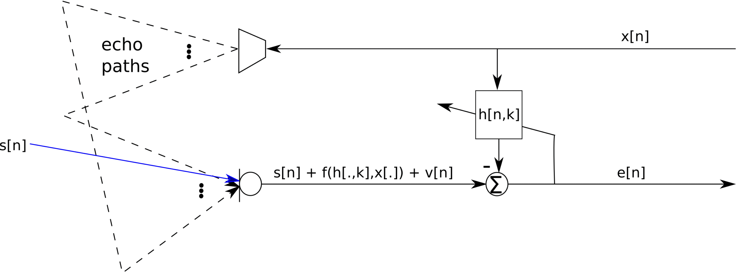
Figure 1: Single line AEC architecture

The problem at hand is to correctly estimate the filter taps, such that $f(h[.],x[.]) = \sum\limits_{i=1}^M h[i]x[k-i]$ , to minimize the error. The presence of the signal $s[n]$ may cause the adaptive system to cancel out the speech signal, thus leading most AECs updating the filter coefficients only when there is no speech detected. Now consider a received signal

$r[k] = \sum\limits_{i=1}^M h[i]x[k-i] + v[k]$

where $v[k]$ is additive noise. Also consider that $x[k-i], \forall i \in \{1, \cdots, M\}, \forall k$ is known. We want to estimate $\hat{h}[i], \forall i \in \{1, \cdots, M\}$ such that $|e[n]|^2$ is minimized, where

$e[n] = \sum\limits_{i=1}^M (h[i]-\hat{h}[i])x[n-i] + v[n]$

Consider the noise signal being i.i.d. Gaussian, then the likelihood function, the joint pdf, for a frame of length N can be given as

$f_{{\bf r}|{\bf h}}({\bf r}|{\bf h}) = \prod\limits_{k=1}^N \frac{1}{\sqrt{2\pi \sigma_{r_k}}} e^{-\frac{\left(r_k-\sum\limits_{m=1}^M h[m]x[k-m] \right)^2}{\sigma_{r_k}^2}}$

where ${\bf r}= [r[1], \cdots,r[N]]^T$ , ${\bf h}= [h[1], \cdots,h[M]]^T$ and $\sigma_{r_k}^2 = \sigma_{v_k}^2, \forall k$ . The log-likelihood function then becomes

$L({\bf r}|{\bf h}) =\kappa -\sum\limits_{k=1}^N \left(\frac{1}{4} \log{\sigma_{v_k}^2} +\frac{\left(r_k-\sum\limits_{m=1}^M h[m]x[k-m] \right)^2}{\sigma_{v_k}^2} \right)$

where $\kappa$ is a constant term. The maximum value of the log-likelihood function will obey:

$\sum\limits_{k=1}^N \frac{2}{\sigma_{v_k}^2} \left(r_k-\sum\limits_{m=1}^M h[m]x[k-m] \right) x[k-q] =0 , q \in \{1,\cdots,M\}$

Thus the ML algorithm will proceed as:

$\hat{h}[i]_{n+1} = \hat{h}[i]_{n} + \mu_i \sum\limits_{k=1}^N \frac{2}{\sigma_{v_k}^2} \left(r_k-\sum\limits_{m=1}^M h[m]x[k-m] \right) x[k-i]$

Comparing the ML update equation to the NLMS algorithm update which is reproduced below,

$\hat{h}[i]_{n+1} = \hat{h}[i]_{n} + \sum\limits_{k=1}^N \left(\frac{1}{\sum\limits_{m=1}^M x[k-m+1]^2 } \left(r_k -\sum\limits_{m=1}^M \hat{h}[m]_{n} x[k-m+1]\right) x[k-i] \right)$

it can be seen that there is a change of $\frac{1}{\sum\limits_{m=1}^M x[k-m+1]^2 }$ to $\frac{2}{\sigma_{v}^2}$ and a reintroduction of the step size $\mu_i$ . The popularity of the NLMS is precisely because of the availability of $\frac{1}{\sum\limits_{m=1}^M x[k-m+1]^2 }$ . However, given a frame size of length $N >> 1$ , the variance of the noise could easily be estimated. Notice that the variance of the noise is the same as that of the recorded signal $r_k$ and if given that $r_k$ is zero mean, then the variance can be estimated directly from $r_k$ . A sample result for this algorithm is shown in Figure 2 below with comparison with the NLMS algorithm.

Figure 2: Performance of ML AEC

VOCAL Technologies offers custom designed solutions for beamforming with a robust voice activity detector, acoustic echo cancellation and noise suppression. Our custom implementations of such systems are meant to deliver optimum performance for your specific beamforming task. Contact us today to discuss your solution!

Complete Communications Engineering

Acoustic echo cancellation with the ML algorithm

More Information